Hyperbolic Geometry 4

Parallel Lines	Models	Geodesics	Circles	Area
Trigonometry	Right Triangles	General Triangles	Rigid Motions	Isometry Group
Möbius Transformations	Poincaré Disk Model	Klein Model	Horocycles	Horocycle Coordinates

Hyperbolic Geometry Continued (Page 4)

The Klein Model

We now take a look at the last model that we will be discussing, the Klein model. Like the Poincaré disk model, the Klein hyperbolic space covers the interior of the unit disk. The metric and geodesics, however, are quite different. For starters, the metric is not conformal; there is a non-zero cross term, so that angles will not be preserved. Any general line element in any space can be written as

metric2

where the $g_{ij}$ are called the metric coefficients or elements of the metric. In the Klein model, the element $g_{12}=g_{21}$ is not 0. Rather, the elements are given as

g11
g11
g22 .

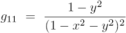
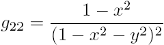From this we can write the full line element:

metrick .

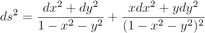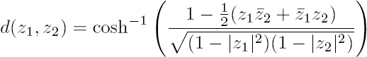
To find a distance function in the Klein model, we see that there is a natural map from the Poincaré disk to the Klein disk. For $z\in\mathbb{H}_D^2$ and $w\in\mathbb{H}_K^2$ , we have that $w=\frac{2z}{1-|z|^2}$ , or $z=\frac{1-\sqrt{1-|w|^2}}{|w|^2}w$ . With this map, we can find that the distance between any two points in the Klein disk is

dist3

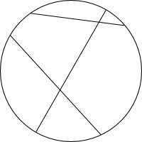
What of the geodesics? It turns out that the geodesics on the Klein disk are chords that cut the boundary, as shown in the figure to the right. Straight lines in this model are actually straight Euclidean lines. The similarity to the disk model, however, should not be forgotten; the geodesics still meet the boundary in the same places, and even the main parameterization looks the same: $x=\tanh r\cos\theta$ , and $y=\tanh r\sin\theta$ .

Now let's make sure that the Gaussian curvature, supposedly an invariant of the space, is the same as with the other models; namely, equal to -1. Because the metric is not conformal, we need to use more advanced differential geometry to obtain the Gaussian curvature. For this, we introduce the Christoffel symbols:

christ

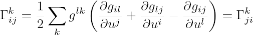
where $(g^{kl})=(g_{ij})^{-1}$ is the inverse matrix of the metric and the are the coordinates of the space ( and , say). The Gaussian curvature is then defined by

gauss2

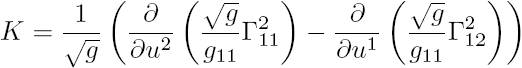
with

christ1

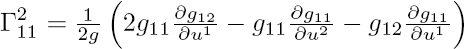
and

christ2

where $g=\det(g_{ij})=g_{11}g_{22}-g_{12}^2$ is the determinant of the metric. When we take the required derivatives and substitute in to find the Gaussian curvature, we find that (big surprise) it is a constant: -1. Hence the Klein model is consistent with the other models of hyperbolic geometry.

Horocycles

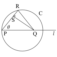
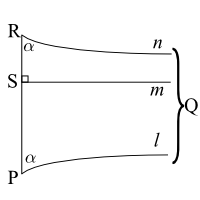
Consider the image to the right drawn in the Poincaré disk, with line a diameter of the disk. Let us consider what happens when we move the point to the right while keeping the distance fixed. The angle $\theta$ will converge to the angle $\alpha$ shown below, the angle of parallelism. This angle is only a function of the distance of point to line . As goes to infinity, it becomes an ideal point on the boundary of the disk, while the segments and become the geodesics and . The circle converges to a horocycle, a curve whose normals converge asymptotically.

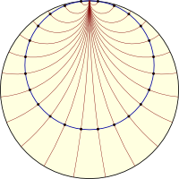
The figure on the right shows a horocycle in blue and some of its normals in red. Notice that the horocycle is tangent to the boundary of the disk, whereas hypercycles would intersect it twice (geodesics being hypercycles orthogonal to the boundary).

In the half-plane model, horocycles are circles tangent to the -axis and horizontal lines, as can be imagined by performing the usual mapping from the disk to the upper half plane. If we imagine a family of horocycles, it is not hard to see that they span the entire hyperbolic space, so that it would make sense to create a set of coordinates from them and the asymptotic lines orthogonal to them.

Horocycle Coordinates

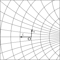
Consider the family of asymptotic lines meeting at an ideal point on the boundary of the unit disk (the point where is crosses the positive real axis, say), like , , and in the above figure, as well as the horocycles orthogonal to them. Let us define a set of coordinates $(\xi,\eta)$ so that $\xi$ measures the horocycle distance from some arbitrary origin (the center of the disk, say) and $\eta$ measures which asymptotic line off of the real axis you are on, as in the figure to the left.

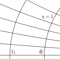
Now let us consider the arc length along horocycle 1 as $s(\xi,\eta)$ . Let of $\eta$ be divided into subintervals (asymptotic lines at $\eta=p/q$ ) with $p=0,\dots,q$ . There is a rotation at infinity (an ideal rotation) that maps each line to the next one leaving the horocycles invariant (the horocycles slide along themselves isometrically). Hence, the horocyclic arc lengths are equal, so $s\left(\xi,\tfrac{p}{q}\right)=\tfrac{p}{q}s(\xi,1)\Rightarrow s(\xi,\eta)=\eta s(\xi,1)$ .

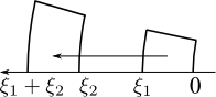
We can also translate along $\xi$ , as shown to the left. It is a remarkable fact that all horocycles are congruent; that is, any one can be mapped into another via an isometry. This implies that

horo6

for (usually so that the horocycles have unit speed).

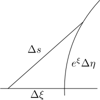
To measure the line element, we use the Pythagorean Theorem as shown in the figure to the right. Hence we have that $ds^2=d\xi^2+e^{2\xi}d\eta^2$ . This is the horocycle metric (line element), which is just another way of representing the Poincaré disk metric in a different set of coordinates. Ergo, the length of any curve can be found using

horogeo

Now let's look for the geodesics in these coordinates. Since the model is still the Poincaré disk, we expect that the geodesics will be the same. We start with the Euler-Lagrange equations for our line element. Let $\phi=\dot{\xi}^2+e^{2\xi}\dot{\eta}^2$ . Then the Euler-Lagrange equations are:

euler .

which implies that

euler2

From these we get that $e^{2\xi}\dot{\eta}=A$ and $A^2e^{-2\xi}-\ddot{\xi}=0$ , which after multiplying by $-2\dot{\xi}$ and integrating yields $A^2e^{-2\xi}+\dot{\xi}^2=B$ . If we choose , then along a geodesic, $\phi=1$ so that

phi2

If $A\neq 0$ , let $\xi_0=\ln A$ so that $\dot{\xi}=\sqrt{1-e^{-2(\xi-\xi_0)}}$ . If we now let $\zeta=e^{\xi-\xi_0}$ , then $\dot{\zeta}=\sqrt{\zeta^2-1}$ , which implies that

archoro

Taking so that $\zeta=\cosh s$ , we find

eta2

In conclusion, the equations for a straight line in horocycles coordinates are

xieta

If we had chosen instead, we would have the equations for the asymptotic lines orthogonal to the horocycles,

xieta2

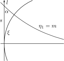
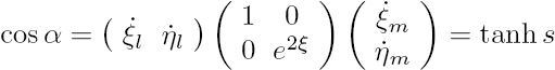
Now consider the figure to the right, where line passes through the origin so that

xieta3

where s is a measure of distance along the line. Then we have that along the line,

xietal

while along the line of constant $\eta$ we have that

xietam

The angle of parallelism, $\alpha$ , can be determined by taking the inner product of these lines:

cosalpha

It is left as an exercise to use this to show that the equation for a horocycle in polar coordinates on the unit disk is $\tanh\frac{r}{2}=\cos\theta$ .

As a final challenge, let us wrap up by coming back to the half plane model and examine what horocycle coordinates look like there. Here we have

xy3

so that the geodesics are

xy2

and

If we rearrange these equations, we get $(x-\eta_0)^2+y^2=(e^{-\xi_0})^2$ and $x=\eta_0$ , exactly the geodesics that we expect in the half plane model. Hence all three models discussed are quite consistent with one another. I hope that this exposé on hyperbolic geometry has been interesting, and I encourage you to read more on the subject.

The Quantum Immortal

Hyperbolic Geometry Continued (Page 4)

The Klein Model

Horocycles

Horocycle Coordinates

Previous Page