Hyperbolic Geometry Continued (Page 3)
Rigid Motions of the Hyperbolic Plane
A rigid motion is a linear transformation from a vector space to itself such that the inner product structure is preserved; that is, lengths, angles and areas are unchanged by the mapping. There are three classes of rigid motions (isometries) of the hyperbolic plane: inversions through a semicircle geodesic, translations parallel to the \(x\)-axis, and reflections about vertical geodesics. This is slightly different from the group of isometries of \(\mathbb{R}^2\), where we have any translation, any reflection about a line, a rotation about a point, and a translation composed with a reflection (a so-called "glide reflection").
We can write the explicit function of each isometry using the complex half plane. An inversion through a semicircle of radius \(k\) is \[I_{C,k}(z)=\frac{k^2}{\bar{z}-a}+a\] with \(C=(a,0)\). Note that an inversion of a polar function \(r=f(\theta)\) centered at the center of the inversion semicircle yields another polar function \(r'=F(\theta)=\frac{k^2}{f(\theta)}\), and that inversions always reverse the orientation of the set upon which it acts (just like a Euclidean reflection). Also, note that two consecutive inversions through different semicircles correspond to a hyperbolic rotation, in that a single point (the intersection of the semicircles) is fixed and orientation is preserved.
The formula for a reflection about a vertical ray with \(x\)-coordinate \(m\) is \(\rho_m(z)=-\bar{z}+2m\), and the expression for a translation parallel to the real axis is \(t_a(z)=z+a\) with \(a\in\mathbb{R}\).
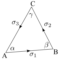
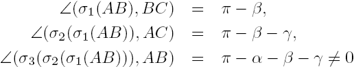
The figure to the right shows that just as two inversions can form a rotation, so can three non-collinear translations. The segment \(AB\) is parallel transported around the triangle is such a way that the angle it makes with the initial segment is non-zero in general (unless the triangle is ideal). Hence, the segment \(AB\) has been rotated by the angle defect of the triangle. Remember, though, that translations not parallel to the real axis are not isometries, and hence are not members of the group of orthogonal transformations of \(\mathbb{H}^2\).
Isometries of the Hyperbolic Plane
Let's examine the group structure of the orientation-preserving isometries of \(\mathbb{H}^2\) (the complete group of isometries, including orientation-reversing ones, is denoted \(\textrm{Isom}(\mathbb{H}^2)\simeq\textrm{PS*L}_2(\mathbb{R})\), where the star indicates that the determinant of the elements of that group may be 1 or -1. For the most case, we only need to deal with orientation-preserving transforms). We denote this group by \(\textrm{PSL}_2(\mathbb{R})=\textrm{SL}_2(\mathbb{R})/{\pm 1}\), known as the projective special linear group of dimension 2 over the real numbers (which is the special linear group modulo the parity group). This group acts on \(\mathbb{H}^2\) as \(\textrm{PSL}_2(\mathbb{R})\hookrightarrow \mathbb{H}^2\) via the complex mapping \(z\mapsto\frac{az+b}{cz+d}\), with \(a,b,c,d\in\mathbb{R}\). These transformations are known as Möbius Transformations, which we discuss in the next section. These transformations only preserve the upper half-plane, though: to map all of \(\mathbb{C}\), we need \(a,b,c,d\in\mathbb{C}\), not just the reals. Hence we have that \(\textrm{PSL}_2(\mathbb{R})\) is the group of conformal automorphisms of the upper half plane \(\mathbb{H}^2\). The action \(\textrm{PSL}_2(\mathbb{R})\hookrightarrow \mathbb{H}^2\) is transitive, so that \(\forall\;z_1,z_2\in\mathbb{H}^2,\;\exists\;g\in\textrm{PSL}_2(\mathbb{R})\) such that \(gz_1=z_2\). It is also faithful, so that if \(gz=z\;\forall\;z\in\mathbb{H}^2\), then \(g=e\), the identity element of \(\textrm{PSL}_2(\mathbb{R})\), which is just the constant 1. We can make an association between the Möbius transformation \(z\mapsto\frac{az+b}{cz+d}\) and the 2x2 matrix \(\begin{pmatrix}a&b\\c&d\end{pmatrix}\). Here we can see the relation to the special linear group: it is required that \(ad-bc=1\). The stabilizer of an element \(z\in\mathbb{H}^2\) is the set \(\{g\in\textrm{PSL}_2(\mathbb{R}):gz=z\}\). This does not automatically mean that \(g\) is 1; for example, the stabilizer of the complex number \(i\) is
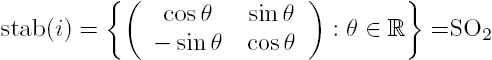
which is just the special orthogonal group of dimension 2. Since the action of \(\textrm{PSL}_2(\mathbb{R})\) on \(\mathbb{H}^2\) is transitive, any \(z\in\mathbb{H}^2\) can be mapped to \(i\) by some \(g\) in the group, and we have the isomorphism \(\textrm{stab}(z)\simeq\textrm{SO}_2\;\forall\;z\in\mathbb{H}^2\), so that \(\mathbb{H}^2\) is actually isomorphic to the quotient group \(\textrm{PSL}_2(\mathbb{R})/\textrm{SO}_2\). Pretty amazing!
Möbius Transformations
Let us now examine more closely the elements of \(\textrm{PSL}_2(\mathbb{R})\) as they relate to the metric and as transforms of \(\mathbb{H}^2\). We already know that \(ad-bc=1\), but let's prove that these are actually isometries, that is, they leave the hyperbolic metric invariant. The Möbius transform \(z\mapsto\frac{az+b}{cz+d}\) can be differentiated and simplified to yield \(dz'=\frac{dz}{(cz+d)^2}\), where \(z'\) is the transformed complex number. Now, \[2iy'=z'-\bar{z}'=\frac{z-\bar{z}'}{(cz+d)(c\bar{z}+d)},\] so that we may make a relation between the primed and unprimed coordinates: \[\frac{dz'\,d\bar{z}'}{(z'-\bar{z}')^2}=\frac{dz\,d\bar{z}}{(z-\bar{z})^2},\] or, when we use \(dx^2+dy^2=dzd\bar{z}\), \[\frac{dx^2+dy^2}{y^2}=\frac{dx'^2+dy'^2}{y'^2}\] so that we can see that Möbius transformations preserve the metric of \(\mathbb{H}^2\), and hence are isometries. Since they preserve distance, we may take the unit-speed geodesic through \(i\) as
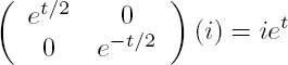
In general, this geodesic can then be mapped to other geodesics by elements of \(\textrm{PSL}_2(\mathbb{R})\) as
The Poincaré Disk Model
We already know that there is a biholomorphic (bijective holomorphic) function that maps the upper half-plane which we now call \(\mathbb{H}_P^2\) to the unit disk \(\mathbb{H}_D^2\) as a consequence of the Riemann Mapping Theorem. In this model (the Poincaré Disk Model), the hyperbolic plane is the set of points lying inside of the unit circle, with the circle itself representing the boundary at infinity. The complex function \(U(z)=\frac{iz+1}{z+i}\) takes the real axis to the unit circle, and the upper half-plane to its interior, while the function \(U^{-1}(z)=V(z)=\frac{iz-1}{-z+i}\) is its inverse. Note that these are both Möbius Transformations, hence it will take geodesics to geodesics and is a conformal mapping. If \(f\) is a rigid motion in \(\mathbb{H}_P^2\), then \(f^*=U\circ f\circ V\) is a rigid motion in \(\mathbb{H}_D^2\), so that rigid motions in the disk model take the form
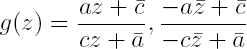
with \(|a|>|c|\).
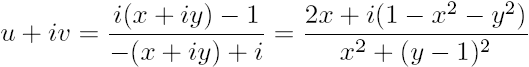
Let's examine the metric on \(\mathbb{H}_D^2\) and get a sense of what geodesics look like in the disk model. Let \(z=x+iy\in\mathbb{H}_D^2\) and \(w=u+iv\in\mathbb{H}_P^2\) so that \(w=V(z)=\frac{iz-1}{-z+i}\). Then we have that
 .
.
By equating the real and imaginary parts, we have that \(u=\frac{2x}{x^2+(y-1)^2}\) and \(v=\frac{1-x^2-y^2}{x^2+(y-1)^2}\). The total differential can be found via \(du=\frac{\partial u}{\partial x}dx+\frac{\partial u}{\partial y}dy\) and a similar expression for \(dv\), with partial derivatives of
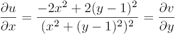
and
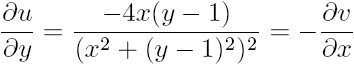
by the Cauchy-Riemann conditions. Hence
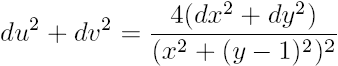
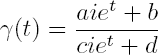
Now let us consider a curve \(\gamma(t)=(x(t),y(t))\) in \(\mathbb{H}_D^2\) and a curve \(\gamma^*(t)=(u(t),v(t))\) in \(\mathbb{H}_P^2\). Because the spaces are isometric,

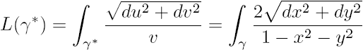
so that the metric can be seen to be
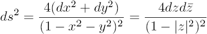
for the Poincaré disk model. As an aside, let us look at a different parameterization. The unit disk model, when the boundary is included, is homeomorphic to the unit disk in ordinary two dimensional space. This suggests that a polar form of hyperbolic coordinates could be used to describe this space. Let the polar coordinates in normal 2D space be \((r,\theta)\) and the hyperbolic coordinates be \((\rho,\theta)\) (clearly the angular dependence is unchanged by symmetry). Then a re-parameterization of the radial distance is given by
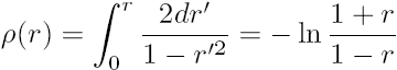
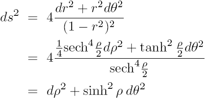
so that \(r=\tanh(\rho/2)\). From ordinary polar theory, we can now write \(x=\tanh(\rho/2)\cos\theta\) and \(y=\tanh(\rho/2)\sin\theta\) and rewrite the metric using \(dr=\tfrac{1}{2}\textrm{sech}^2\tfrac{\rho}{2}d\rho\) and \(dr^2=\tfrac{1}{4}\textrm{sech}^4\tfrac{\rho}{2}d\rho^2\):
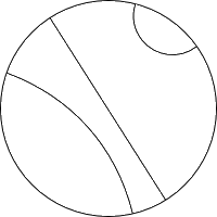
We are now ready to examine the shape of geodesics in \(\mathbb{H}_D^2\). Again due to the isometric nature of the Möbius map between the models, we can apply our transformation to the geodesics of the half-plane to obtain geodesics on the disk. We can see that the geodesics on the disk are arcs of circles perpendicular to the boundary of the disk, as well as diameters. The diameters correspond to the vertical ray geodesics of the half-plane model, while the arcs orthogonal to the boundary are the transforms of the semicircles centered on the \(x\)-axis. It is important to note that the boundary of the disk itself is not part of the hyperbolic space, but can be included in a compactified region just as the point at infinity can be included in the stereographic projection of the complex plane. Hypercycles in the disk model are then arcs of circles that cross the boundary (not necessarily at 90 degrees).
Let us look at how we might obtain a formula for the distance between two points in \(\mathbb{H}_D^2\). We start by noting that for any curve in the disk, we can parameterize it by \(z(t)=x(t)+iy(t)\), so that
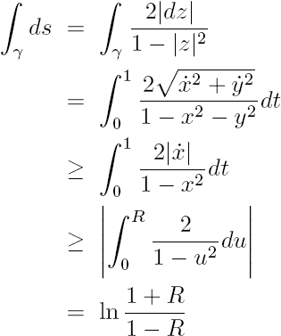
hence the hyperbolic distance along a diameter of the disk is \(d(0,R)=\ln\tfrac{1+R}{1-R}\). Now let's look at the map \(\phi(z)=\frac{z-z_1}{1-\bar{z}_1z}\in\textrm{Aut}(\mathbb{H}_D^2)\), which maps the disk to itself and hence is a member of the group of automorphisms on the disk. Because it is a Möbius transformation, it is an isometry, and we see that it maps \(z_1\mapsto 0,z_2\mapsto\frac{z_2-z_1}{1-\bar{z}_1z_2}\), so that
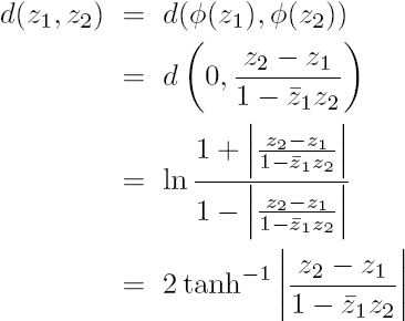
where we have used the relation \(\tanh^{-1}x=\tfrac{1}{2}\ln\left(\tfrac{1+x}{1-x}\right)\).
It would now be instructive to discuss Gaussian curvature and it's relation to hyperbolic space. While the complete definition of Gaussian curvature is rather technical, we can say that it is an intrinsic measure of how a surface is curving, independent of the space in which it is embedded. To find the Gaussian curvature of hyperbolic space in these various models, we first consider the notion of a conformal metric. This is a metric which can be written as \(ds=\lambda(z)|dz|\), so that the arc length is directly proportional to the Euclidean metric through some function of z. For the disk model, we have \(\lambda(z)=\frac{2}{1-|z|^2}\), while for the half plane we have \(\lambda(z)=\frac{2i}{z-\bar{z}}\). If the metric is conformal, we can immediately compute the Gaussian curvature of the space using \(K=-\frac{\nabla^2\ln\lambda}{\lambda^2}\), where we use \(\nabla^2=\frac{\partial^2}{\partial x^2}+\frac{\partial^2}{\partial y^2}=4\frac{\partial}{\partial z}\frac{\partial}{\partial\bar{z}}\). It is easy to compute \(K\) for the two Poincaré models discussed thus far, and we see that the Gaussian curvature is a constant -1. The fact that it is constant means that the curvature is the same at every point in space, and the fact that it is negative means that the surface curves inward (like a saddle) at every point. It is a remarkable fact that no matter how you model or parameterize the space, the Gaussian curvature does not change, and can be computed solely from the metric.
Previous Page |
Next Page |